Blog Writing Guidelines

Welcome to the DSPG Quarto blog. This post will be a demonstration of some of the capabilities of a quarto doc and some basics of dos and don’ts as you’re writing your own blogs throughout the DSPG program.

RMarkdown and Quarto Markdown

These blogs are generated using Quarto Markdown (.qmd). Markdown is a special type of text format that is both legible with and without its rendering. Quarto Markdown follows the syntax of basic Markdown and has some additional features for use as well. The Markdown Basics guide on the Quarto page will be a great resource to view how you can format your texts.

Yaml Headers

Each blog has its own yaml style metadata section at the top of the file. This one has a metadata section that looks something like this in the source code.

---
title: "Blog Writing Guidelines"  # The title of your post
author: "Harun Celik"             # The author associated with the blog post
date: "2024-05-05"                # The date in Year-Month-Day format
categories: [blog tutorial]       # The categories associated with the blog
---

There are additional options for the yaml that you can check out through the Quarto documentation page.

Linking Pages and Images

You can link items in your files by using the following syntax [Text of Link](Link Reference - URL). Referencing also works for adding images into your blogs. The syntax is very similar, but requires an ! in the front. So an example would be ![Stock Photo of a Data Cat](imgs/Data_Cat.png)

Since this post doesn’t specify an explicit image in the yaml, the first image in the post will be used as the thumbnail of the post. A couple of things to remember with linking images.

Place your images in the imgs directory. This helps prevent clutter and makes it easier to find the files.
Name your images explicitly. Don’t call them "image_1.jpg" but instead something like "age_scatterplot_1".
Don’t save file names with any spaces. Add an _ or use camelCaseNaming. Spaces will prevent the blog from properly rendering!
Make sure you follow copyright guidelines on images. Don’t add images you would not be permitted to share in any professional environment.

Running Code

Code Chunks

One of the coolest features of the Quarto blogs is the ability to integrate code chunks and have them render. Let’s check out how this works. Here is an example of what a code chunk looks like in the source code.

print("I would like for this text to print.")

[1] "I would like for this text to print."

Using different markdown arguments, we can customize our code chunks to prevent them from running, displaying, or rendering messages. You can check out some of those options through the R Markdown Reference Guide.

Some useful ones are below.

eval=TRUE      # If FALSE, knitr will not run the code in the code chunk.
include=TRUE   # If FALSE, knitr will run the chunk but not include the chunk in the final document.
echo=TRUE      # If FALSE, knitr will not display the code in the code chunk above it’s results in the final document.
message=TRUE   # If FALSE, knitr will not display any messages generated by the code.
warning=TRUE   # If FALSE, knitr will not display any warning messages generated by the code

Using Data

Most of the time, you’ll want to run some code that generates a table or a visual of your data. To do this, quarto will need a local reference to your data and that’s why your blogs also come with a directory labelled data\. If you are working within R, it is advisable to use the .RDS format for saving any data you want to use for displaying code. Let’s look at an example.

# Let's create a data frame to use

## Generate pay grades as factors
Grades <- c("Grade A", "Grade B", "Grade C", "Grade D", "Grade E")
Grades_Factor <- factor(Grades, levels = c("Grade A", "Grade B", "Grade C", "Grade D", "Grade E"))

# Create randomized vectors of size 50
Gender <- sample(x = c("Woman", "Man", "Transgender", "Non-binary/non-conforming", "Prefer not to respond"), size=50, replace = TRUE)
ID <- sample(x = 1000:3000, size=50)
Pay <- sample(x = Grades_Factor, size=50, replace=TRUE)

# Create data frame
df <- data.frame(Gender, ID, Pay)

In our example here we’ve created the data in our blog environment, but often this will not be the case. We are going to pretend that our data is stored in the data directory. We will first save the data we created.

# Saving our dataset
saveRDS(df, file = "data/PayData.RDS")

Now we can load it in as Pay_DF.

Pay_DF <- readRDS("data/PayData.RDS")

Let’s write some code with ggplot2 to create a visual.

library(ggplot2)

pay_colors <- c("Grade A" = "#1f78b4", "Grade B" = "#33a02c", "Grade C" = "#e31a1c", "Grade D" = "#ff7f00", "Grade E" = "#6a3d9a")

ggplot(Pay_DF, aes(x = Gender, fill = Pay)) +
  geom_bar() +
  labs(x = "Gender", y = "Count", title = "Distribution of Pay Grades Across Genders") +
  scale_fill_manual(values = pay_colors) +
  theme_minimal() +
  coord_flip()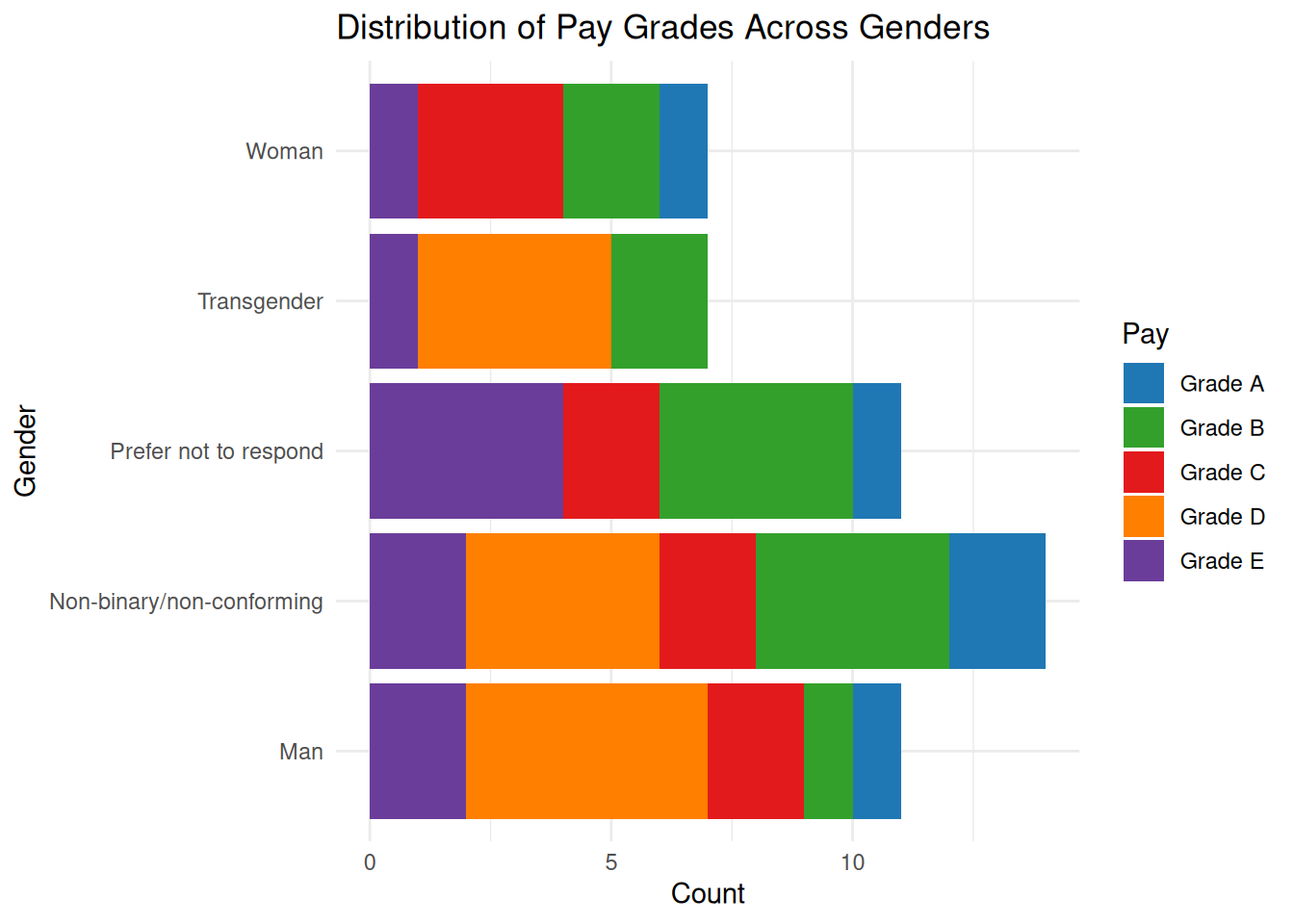

Data Guidelines

Here are some important things to consider when you’re using data sets in your blogs.

VERY IMPORTANT: All data saved in the data directory is publicly visible. Don’t share data that is private into your blogs.
Be mindful of the size of your data. The larger the data, the longer it will take to render. GitHub also limits commit sizes so keep this in mind.

Using Other Languages

The last thing we will look at is displaying code for languages other than R. RMarkdown files have the ability to change the rendering engine so that other languages can also be used. To run Python, you will have to have the reticulate library installed and configured. When you’ve created a code chunk, you will want to switch the section that is typically in the form of {r} to {python} or whatever other supported language you wish to use.

Here is a Python code block.

import platform

print("This code is run using python version", platform.python_version())

This code is run using python version 3.12.3